Refractive Geometry
AquaCal models the optical path of light rays traveling from underwater calibration targets, through the air-water interface, and into cameras positioned above the water. Understanding this refractive geometry is essential for interpreting how the calibration works and why it differs from standard pinhole calibration.
Physical Setup
In a typical AquaCal calibration setup, an array of cameras is mounted in air (near Z ≈ 0), pointing downward at a flat water surface (Z = water_z). A calibration board sits underwater (Z > water_z). Light from board corners travels upward through water, refracts at the interface, continues through air, and enters the cameras.
The key physical insight: light bends at the interface. A straight ray in water becomes a bent ray when viewed from air, and vice versa. This refraction changes the apparent position of underwater points when viewed from above.
Snell’s Law
Snell’s law governs how light bends when crossing the boundary between two media with different refractive indices.
Scalar Form
The classic scalar form relates the angles of incidence and refraction:
where:
\(n_{\text{air}} \approx 1.000\) (refractive index of air)
\(n_{\text{water}} \approx 1.333\) (refractive index of water)
\(\theta_i\) is the angle between the incident ray and the surface normal
\(\theta_r\) is the angle between the refracted ray and the surface normal
3D Vector Form
AquaCal uses the 3D vector form of Snell’s law, which operates on ray directions rather than angles:
where:
\(\mathbf{d}\) is the unit incident ray direction
\(\mathbf{t}\) is the unit refracted ray direction
\(\mathbf{n}\) is the surface normal (oriented to point into the destination medium)
\(\eta = n_1 / n_2\) is the refractive index ratio
\(\cos\theta_i = |\mathbf{d} \cdot \mathbf{n}|\)
\(\cos\theta_t = \sqrt{1 - \eta^2(1 - \cos^2\theta_i)}\)
The implementation handles the normal orientation automatically. See aquacal.core.refractive_geometry.snells_law_3d() for the full implementation.
Visualizing Refraction
The diagram below shows a cross-section of a ray path from a camera in air to an underwater target:
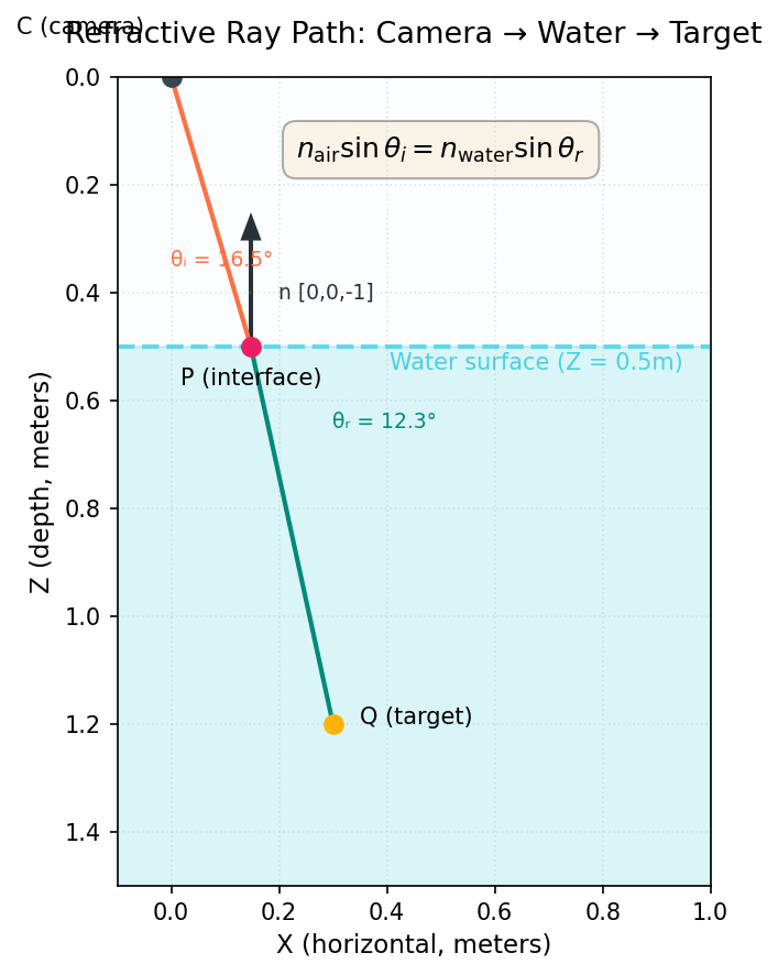
Key observations:
The incident ray (red) travels from the camera C downward through air toward the interface
At point P on the interface, the ray refracts according to Snell’s law
The refracted ray (green) continues through water to reach the underwater target Q
The interface normal n points upward (from water toward air: [0, 0, -1])
The incident angle \(\theta_i\) is larger than the refracted angle \(\theta_r\) because light entering a denser medium bends toward the normal
Gotcha: Interface Normal Direction
The interface normal is defined as [0, 0, -1], which points upward (from water toward air). This is the outward normal when viewed from the water side. The sign might seem counterintuitive given the Z-down world frame, but it’s consistent with the “outward from denser medium” convention.
The snells_law_3d() function handles normal orientation internally, so you don’t need to flip it manually depending on ray direction.
Ray Tracing Through the Interface
Given a camera position C in air and an underwater target point Q, how do we find where the light ray crosses the interface?
The 1D Snell Equation
The problem reduces to finding the interface crossing point P where Snell’s law is satisfied. Due to rotational symmetry about the vertical axis through C, this becomes a 1D root-finding problem for the horizontal distance \(r_p\) from C to P:
where:
\(\sin\theta_{\text{air}} = r_p / \sqrt{r_p^2 + h_c^2}\)
\(\sin\theta_{\text{water}} = (r_q - r_p) / \sqrt{(r_q - r_p)^2 + h_q^2}\)
\(h_c = \text{water_z} - C_z\) is the camera-to-interface gap
\(h_q = Q_z - \text{water_z}\) is the interface-to-point gap
\(r_q = \|\mathbf{Q}_{xy} - \mathbf{C}_{xy}\|\) is the horizontal offset between camera and target
This function is strictly monotonic and crosses zero exactly once in the interval \((0, r_q)\), guaranteeing a unique solution.
Newton-Raphson Solution
AquaCal uses Newton-Raphson iteration to solve for \(r_p\):
Initial guess: Use the pinhole/straight-line approximation: \(r_p = r_q \cdot h_c / (h_c + h_q)\)
Update: \(r_p \leftarrow r_p - f(r_p) / f'(r_p)\)
Convergence: Typically 2-4 iterations achieve sub-micrometer accuracy
The derivative \(f'(r_p)\) has a closed form, making the iteration very fast. Once \(r_p\) converges, the interface point is:
This Newton-Raphson approach is ~50× faster than bracketing methods like Brent’s method, while maintaining excellent numerical stability. See aquacal.core.refractive_geometry.refractive_project() for the implementation.
Gotcha: water_z is a Z-coordinate, not a distance
Despite its name, the water_z parameter in AquaCal is actually the Z-coordinate of the water surface in the world frame (the value of water_z), not the physical distance from a camera to the water.
The physical camera-to-water gap \(h_c\) is computed internally as water_z - C_z, where C_z is the camera’s Z position in world coordinates.
For the reference camera at the world origin (C_z = 0), the water_z equals the physical gap. For other cameras at slightly different heights, the gap differs, but all cameras share the same water_z value (the global water surface Z).
This reparameterization eliminates a mathematical degeneracy between camera Z position and interface distance. See the Optimizer Pipeline page for details.
Projection Model
Forward Projection: 3D Point → Pixel
Given an underwater 3D point Q in world coordinates, how does it project to a pixel in a camera image?
Standard pinhole projection (no refraction) simply transforms Q to camera coordinates, then applies the camera intrinsics:
Refractive projection accounts for the bent light path:
Solve for the interface crossing point P using the Newton-Raphson method above
Project P (not Q) through the standard pinhole model
This works because the camera observes the air segment of the refracted ray, which travels from C through P. Any point on this segment (including P itself) projects to the same pixel.
The refractive projection is implemented in refractive_project() and vectorized in refractive_project_batch().
When Refraction Matters
Refraction effects are most significant when:
Depth is large: Targets far below the water surface
Off-axis viewing: Cameras viewing at steep angles (large horizontal offset)
High-precision applications: Sub-millimeter 3D reconstruction
For shallow water (~10cm depth) and near-vertical viewing, pinhole projection is often adequate. But for typical AquaCal setups with 0.5-2m underwater depth and wide camera arrays, ignoring refraction introduces systematic depth-dependent bias that grows with distance from the rig center.
See the Optimizer Pipeline page for more on when to use refractive vs. standard calibration.
See Also
Coordinate Conventions — World frame, camera frame, and interface normal definitions
Optimizer Pipeline — How refractive projection fits into the calibration pipeline
aquacal.core.refractive_geometry— API reference for projection and ray tracing functions