Why Refractive Calibration Matters

Underwater imaging systems view targets through a flat air-water interface. A standard pinhole camera model ignores refraction at this interface, treating light as travelling in a straight line from camera to target. AquaCal corrects this using Snell’s law.

But does it actually matter? This tutorial answers that question with three controlled synthetic experiments:

1. Parameter Fidelity — Can both models fit the data? Which one recovers correct parameters?

2. Depth Generalization — Using the same calibration, how does 3D reconstruction accuracy vary with depth?

3. XY vs Z Anisotropy — How does reconstruction precision differ between lateral (XY) and depth (Z) directions?

Because we control all ground truth parameters, we can measure exactly where each model fails and why.

# Colab setup — clones the repo and installs AquaCal if running on Google Colab.
# This notebook imports test helpers from the repo's tests/ directory, so a full
# clone is needed (not just pip install). When running locally, this cell is a no-op.
import sys
from pathlib import Path

if "google.colab" in sys.modules:
    import os
    if not os.path.exists("/content/AquaCal/src"):
        print("Colab detected — cloning repo and installing AquaCal...")
        !git clone --depth 1 https://github.com/tlancaster6/AquaCal.git /content/AquaCal
        !pip install -q -e /content/AquaCal
    else:
        print("AquaCal repo already present.")
    os.chdir("/content/AquaCal")
    print("Done.")
else:
    print("Local environment — skipping install.")

Local environment — skipping install.

# Toggle rig size:
#   "small" — 4 cameras, 20 frames, ideal conditions. Fast, ~2 min total.
#   "large" — 12 cameras, 30 frames, realistic noise. Compelling results, ~60 min total.
RIG_SIZE = "large"

OUTPUT_DIR = Path("output")  # exported data artifacts

Setup and Imports

import sys
from pathlib import Path

import cv2
import matplotlib.pyplot as plt
import numpy as np
import pandas as pd

# Make sure project root is on path (needed when running as a notebook)
_project_root = Path().resolve()
while _project_root.name and not (_project_root / "src").exists():
    _project_root = _project_root.parent
if str(_project_root) not in sys.path:
    sys.path.insert(0, str(_project_root))

from aquacal.config.schema import BoardConfig, InterfaceParams
from aquacal.core.board import BoardGeometry
from aquacal.validation.reconstruction import triangulate_charuco_corners
from aquacal.validation.reprojection import compute_reprojection_errors
from tests.synthetic.experiment_helpers import (
    calibrate_synthetic,
    compute_per_camera_errors,
    evaluate_reconstruction,
)
from tests.synthetic.ground_truth import (
    SyntheticScenario,
    create_scenario,
    generate_dense_xy_grid,
    generate_real_rig_array,
    generate_real_rig_trajectory,
    generate_synthetic_detections,
)

# Consistent color palette for all plots
COLOR_REFRACTIVE = "#2196F3"      # Blue
COLOR_NON_REFRACTIVE = "#F44336"  # Red
LABEL_REFRACTIVE = "Refractive (AquaCal)"
LABEL_NON_REFRACTIVE = "Non-refractive (pinhole)"

print("Imports complete.")

Imports complete.

Preset Configuration

The "small" preset uses the "ideal" scenario: 4 cameras arranged in a grid, near the water surface (15 cm above), boards at 0.25–0.45 m depth, no noise. This is fast and lets you verify the math.

The "large" preset uses the "realistic" scenario: 12 cameras with positions matching the real AquaCal hardware rig (idealized: common intrinsics, optical axes aligned to Z), water surface at ~1.03 m, boards at 1.1–2.0 m depth, 0.5 px noise. This produces compelling quantitative results.

if RIG_SIZE == "small":
    # create_scenario("ideal"): 4 cameras at Z=0, water at Z=0.15, boards at Z=0.25-0.45m
    # All test/sweep depths must be > 0.15m (below water surface)
    SCENARIO_NAME = "ideal"
    TEST_DEPTHS = [0.22, 0.28, 0.35, 0.42, 0.50]
    N_GRID = 4  # smaller grid for 4-camera rig
    XY_EXTENT = 0.05
    XY_CENTER = (0.0, 0.0)
    TILT_DEG = 2.0
else:
    # create_scenario("realistic"): 12 cameras, water at ~1.03m, boards at 1.1-2.0m depth
    SCENARIO_NAME = "realistic"
    TEST_DEPTHS = [1.10, 1.20, 1.30, 1.40, 1.50, 1.70, 2.00, 2.50]
    N_GRID = 7
    XY_EXTENT = 0.5
    XY_CENTER = (-0.34, 0.55)  # centroid of the 12-camera array
    TILT_DEG = 3.0

print(f"RIG_SIZE = {RIG_SIZE!r}")
print(f"  Scenario:    {SCENARIO_NAME}")
print(f"  Test depths: {TEST_DEPTHS}")

RIG_SIZE = 'large'
  Scenario:    realistic
  Test depths: [1.1, 1.2, 1.3, 1.4, 1.5, 1.7, 2.0, 2.5]

Experiment 1: Parameter Fidelity

Question: When we calibrate both models on identical data, do they recover the correct camera parameters?

We generate a synthetic scenario with known ground truth, then run the full calibration pipeline twice — once with the refractive model (n_water = 1.333) and once with the non-refractive pinhole approximation (n_water = 1.0). Both optimizations minimize reprojection error on the same 2D observations.

The key insight: a model can fit 2D observations without learning correct 3D geometry. If the model is wrong, it will compensate by adjusting focal length and camera positions.

print("=== Experiment 1: Parameter Fidelity ===")
scenario = create_scenario(SCENARIO_NAME, seed=42)
print(f"Scenario: {scenario.description}")
print(f"  Cameras: {len(scenario.intrinsics)}")
print(f"  Frames:  {len(scenario.board_poses)}")
print(f"  Noise:   {scenario.noise_std} px")

print("\nCalibrating refractive model (n_water=1.333)...")
result_refr, _ = calibrate_synthetic(scenario, n_water=1.333, refine_intrinsics=True)
errors_refr = compute_per_camera_errors(result_refr, scenario)
print(f"  Reprojection RMS: {result_refr.diagnostics.reprojection_error_rms:.4f} px")

print("\nCalibrating non-refractive model (n_water=1.0)...")
result_nonrefr, _ = calibrate_synthetic(scenario, n_water=1.0, refine_intrinsics=True)
errors_nonrefr = compute_per_camera_errors(result_nonrefr, scenario)
print(f"  Reprojection RMS: {result_nonrefr.diagnostics.reprojection_error_rms:.4f} px")

print("\nBoth calibrations complete.")
print(f"  Note: similar reprojection errors ({result_refr.diagnostics.reprojection_error_rms:.3f} vs "
      f"{result_nonrefr.diagnostics.reprojection_error_rms:.3f} px) — "
      "look at parameter errors next.")

# Interface distance (water_z) recovery — refractive model only
gt_wz = np.mean(list(scenario.water_zs.values()))
est_wz = np.mean([c.water_z for c in result_refr.cameras.values()])
wz_err_mm = (est_wz - gt_wz) * 1000
wz_err_pct = (est_wz - gt_wz) / gt_wz * 100
print(f"\nInterface distance (water_z) recovery [refractive model only]:")
print(f"  Ground truth: {gt_wz * 1000:.1f} mm")
print(f"  Estimated:    {est_wz * 1000:.1f} mm")
print(f"  Error:        {wz_err_mm:+.2f} mm ({wz_err_pct:+.3f}%)")

# Calibration depth range (for Experiment 2 plots)
_board_zs = [bp.tvec[2] for bp in scenario.board_poses]
CALIB_DEPTH_RANGE = (min(_board_zs), max(_board_zs))
print(f"\nCalibration depth range: ({CALIB_DEPTH_RANGE[0]:.2f}, {CALIB_DEPTH_RANGE[1]:.2f}) m")

=== Experiment 1: Parameter Fidelity ===
Scenario: 12-camera rig matching real hardware (idealized geometry)
  Cameras: 12
  Frames:  30
  Noise:   0.5 px

Calibrating refractive model (n_water=1.333)...
Stage 2: Extrinsic initialization...
Stage 3: Joint refractive optimization...
`ftol` termination condition is satisfied.
Function evaluations 17, initial cost 3.3111e+04, final cost 3.4102e+03, first-order optimality 2.31e-03.
Stage 4: Intrinsic refinement...
`ftol` termination condition is satisfied.
Function evaluations 21, initial cost 3.4102e+03, final cost 3.4054e+03, first-order optimality 1.50e+01.
  Reprojection RMS: 0.4984 px

Calibrating non-refractive model (n_water=1.0)...
Stage 2: Extrinsic initialization...
Stage 3: Joint refractive optimization...
`xtol` termination condition is satisfied.
Function evaluations 42, initial cost 1.2535e+05, final cost 2.7124e+04, first-order optimality 4.26e-03.
Stage 4: Intrinsic refinement...
`xtol` termination condition is satisfied.
Function evaluations 19, initial cost 2.7124e+04, final cost 1.5486e+04, first-order optimality 2.57e-03.
  Reprojection RMS: 1.3764 px

Both calibrations complete.
  Note: similar reprojection errors (0.498 vs 1.376 px) — look at parameter errors next.

Interface distance (water_z) recovery [refractive model only]:
  Ground truth: 1031.0 mm
  Estimated:    1032.2 mm
  Error:        +1.19 mm (+0.115%)

Calibration depth range: (1.13, 1.87) m

Focal Length Recovery

When refraction bends rays at the interface, a non-refractive model compensates by adjusting focal length. The result: a systematically biased focal length that happens to minimize 2D reprojection error but does not match the true optics.

camera_names = sorted(scenario.intrinsics.keys(), key=lambda s: int(s.replace("cam", "")))
x = np.arange(len(camera_names))
width = 0.35

focal_refr = [errors_refr[cam]["focal_length_error_pct"] for cam in camera_names]
focal_nonrefr = [errors_nonrefr[cam]["focal_length_error_pct"] for cam in camera_names]

fig, ax = plt.subplots(figsize=(10, 5))
ax.bar(x - width / 2, focal_refr, width, label=LABEL_REFRACTIVE, color=COLOR_REFRACTIVE)
ax.bar(x + width / 2, focal_nonrefr, width, label=LABEL_NON_REFRACTIVE, color=COLOR_NON_REFRACTIVE)
ax.set_xlabel("Camera")
ax.set_ylabel("Focal Length Error (%)")
ax.set_title("Focal Length Recovery Error vs Ground Truth")
ax.set_xticks(x)
ax.set_xticklabels(camera_names, rotation=45, ha="right")
ax.axhline(0, color="black", linewidth=0.5, linestyle="--")
ax.legend()
ax.grid(axis="y", alpha=0.3)
plt.tight_layout()
plt.show()
plt.close()

mean_focal_refr = np.mean([abs(e) for e in focal_refr])
mean_focal_nonrefr = np.mean([abs(e) for e in focal_nonrefr])
print(f"Mean absolute focal length error:")
print(f"  Refractive:     {mean_focal_refr:.3f}%")
print(f"  Non-refractive: {mean_focal_nonrefr:.3f}%")

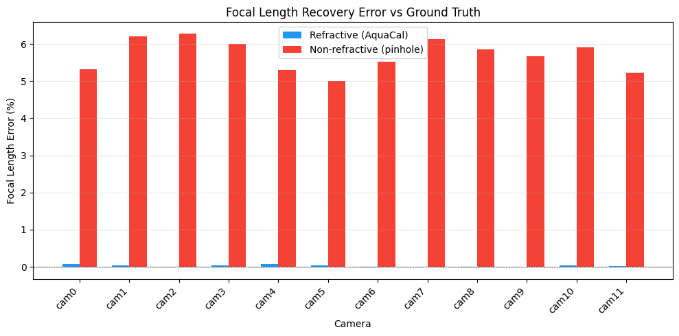
Mean absolute focal length error:
  Refractive:     0.033%
  Non-refractive: 5.699%

Camera Z Position Recovery

Along with focal length, the non-refractive model misplaces camera positions along the Z axis (depth). These two biases together produce a model that fits 2D projections but triangulates 3D positions incorrectly.

Because the reference camera (cam0) is fixed at the world-frame origin during optimization, its raw Z error is always zero by construction. To reveal the systematic shift the model would have applied to the entire rig, we subtract the mean Z error of the free cameras from all cameras (mean-shift correction).

z_refr_raw = [errors_refr[cam]["z_position_error_mm"] for cam in camera_names]
z_nonrefr_raw = [errors_nonrefr[cam]["z_position_error_mm"] for cam in camera_names]

# The reference camera (cam0) is pinned at ground truth during optimization,
# so its raw error is always 0. To reveal the systematic Z shift the model
# would have applied to cam0, subtract the mean error of the free cameras
# from all cameras. This gives each camera's estimated distance from its
# true position, including the reference.
ref_cam = camera_names[0]
free_cams = camera_names[1:]

mean_z_refr = np.mean([errors_refr[cam]["z_position_error_mm"] for cam in free_cams])
mean_z_nonrefr = np.mean([errors_nonrefr[cam]["z_position_error_mm"] for cam in free_cams])

z_refr = [v - mean_z_refr for v in z_refr_raw]
z_nonrefr = [v - mean_z_nonrefr for v in z_nonrefr_raw]

fig, ax = plt.subplots(figsize=(10, 5))
ax.bar(x - width / 2, z_refr, width, label=LABEL_REFRACTIVE, color=COLOR_REFRACTIVE)
ax.bar(x + width / 2, z_nonrefr, width, label=LABEL_NON_REFRACTIVE, color=COLOR_NON_REFRACTIVE)
ax.set_xlabel("Camera")
ax.set_ylabel("Z Position Error (mm)")
ax.set_title("Camera Z Position Recovery Error (mean-shift corrected)")
ax.set_xticks(x)
ax.set_xticklabels(camera_names, rotation=45, ha="right")
ax.axhline(0, color="black", linewidth=0.8, linestyle="--")
ax.legend()
ax.grid(axis="y", alpha=0.3)
plt.tight_layout()
plt.show()
plt.close()

mean_z_refr_abs = np.mean([abs(e) for e in z_refr])
mean_z_nonrefr_abs = np.mean([abs(e) for e in z_nonrefr])
print(f"Mean absolute Z position error (mean-shift corrected):")
print(f"  Refractive:     {mean_z_refr_abs:.2f} mm")
print(f"  Non-refractive: {mean_z_nonrefr_abs:.2f} mm")

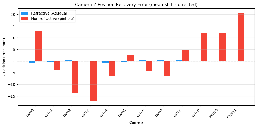
Mean absolute Z position error (mean-shift corrected):
  Refractive:     0.35 mm
  Non-refractive: 9.66 mm

Camera XY Position Recovery

Top-down view of camera positions. Arrows show how far each estimated position is from ground truth. A good calibration produces very short arrows.

fig, ax = plt.subplots(figsize=(8, 8))

for i, cam_name in enumerate(camera_names):
    C_gt = scenario.extrinsics[cam_name].C
    C_refr = result_refr.cameras[cam_name].extrinsics.C
    C_nonrefr = result_nonrefr.cameras[cam_name].extrinsics.C

    gt_label = "Ground Truth" if i == 0 else None
    refr_label = LABEL_REFRACTIVE if i == 0 else None
    nonrefr_label = LABEL_NON_REFRACTIVE if i == 0 else None

    ax.scatter(C_gt[0], C_gt[1], color="black", s=120, zorder=3, label=gt_label, marker="o")
    ax.scatter(C_refr[0], C_refr[1], color=COLOR_REFRACTIVE, s=60, zorder=4, label=refr_label, alpha=0.8)
    ax.scatter(C_nonrefr[0], C_nonrefr[1], color=COLOR_NON_REFRACTIVE, s=60, zorder=4, label=nonrefr_label, alpha=0.8)

    dx_refr = C_refr[0] - C_gt[0]
    dy_refr = C_refr[1] - C_gt[1]
    dx_nonrefr = C_nonrefr[0] - C_gt[0]
    dy_nonrefr = C_nonrefr[1] - C_gt[1]

    arrow_kw = dict(head_width=0.015, head_length=0.008, length_includes_head=True)
    ax.arrow(C_gt[0], C_gt[1], dx_refr, dy_refr, color=COLOR_REFRACTIVE, alpha=0.6, **arrow_kw)
    ax.arrow(C_gt[0], C_gt[1], dx_nonrefr, dy_nonrefr, color=COLOR_NON_REFRACTIVE, alpha=0.6, **arrow_kw)

ax.set_xlabel("X Position (m)")
ax.set_ylabel("Y Position (m)")
ax.set_title("Camera XY Position Recovery (arrows = estimation error)")
ax.set_aspect("equal")
ax.legend()
ax.grid(alpha=0.3)
plt.tight_layout()
plt.show()
plt.close()

mean_xy_refr = np.mean([errors_refr[cam]["xy_position_error_mm"] for cam in camera_names])
mean_xy_nonrefr = np.mean([errors_nonrefr[cam]["xy_position_error_mm"] for cam in camera_names])
print(f"Mean XY position error:")
print(f"  Refractive:     {mean_xy_refr:.2f} mm")
print(f"  Non-refractive: {mean_xy_nonrefr:.2f} mm")

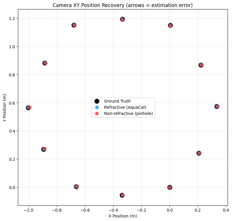
Mean XY position error:
  Refractive:     0.47 mm
  Non-refractive: 4.94 mm

Experiment 1 Takeaway

Both models achieve similar reprojection error — the 2D fitting quality looks the same. But the non-refractive model absorbs the refraction effect into systematically biased focal lengths and camera positions. The refractive model recovers the true physical parameters.

Why it matters: Biased parameters produce systematic 3D reconstruction errors that grow with depth — exactly what Experiment 2 will show.

Experiment 2: Depth Generalization

Question: How does 3D reconstruction accuracy vary with depth for each model?

Real underwater surveys rarely stay at exactly the calibration depth. Fish tracking systems follow animals at varying depths; coral surveys cover different depth strata.

Using the same calibrations from Experiment 1, we evaluate 3D reconstruction accuracy at a range of individual test depths. The refractive model should perform consistently because it learned the correct geometry; the non-refractive model’s biased parameters produce depth-dependent errors.

print("=== Experiment 2: Depth Generalization ===")
print(f"Using calibrations from Experiment 1")
print(f"  Refractive RMS:     {result_refr.diagnostics.reprojection_error_rms:.4f} px")
print(f"  Non-refractive RMS: {result_nonrefr.diagnostics.reprojection_error_rms:.4f} px")
print(f"Test depths: {TEST_DEPTHS}")

board_exp2 = BoardGeometry(scenario.board_config)
print("\nEvaluating at test depths...")

=== Experiment 2: Depth Generalization ===
Using calibrations from Experiment 1
  Refractive RMS:     0.4984 px
  Non-refractive RMS: 1.3764 px
Test depths: [1.1, 1.2, 1.3, 1.4, 1.5, 1.7, 2.0, 2.5]

Evaluating at test depths...

results_refr_exp2 = []
results_nonrefr_exp2 = []
# Save intermediates for Experiment 3 (XY vs Z anisotropy)
exp2_test_poses = []
exp2_test_detections = []

for depth in TEST_DEPTHS:
    print(f"  Evaluating Z = {depth:.2f} m...")

    test_poses = generate_dense_xy_grid(
        depth=depth,
        n_grid=N_GRID,
        xy_extent=XY_EXTENT,
        xy_center=XY_CENTER,
        tilt_deg=TILT_DEG,
        frame_offset=1000,
        seed=42 + int(depth * 100),
    )

    test_detections = generate_synthetic_detections(
        intrinsics=scenario.intrinsics,
        extrinsics=scenario.extrinsics,
        water_zs=scenario.water_zs,
        board=board_exp2,
        board_poses=test_poses,
        noise_std=scenario.noise_std,
        seed=42 + int(depth * 100),
    )

    exp2_test_poses.append(test_poses)
    exp2_test_detections.append(test_detections)

    err_refr = evaluate_reconstruction(result_refr, board_exp2, test_detections)
    err_nonrefr = evaluate_reconstruction(result_nonrefr, board_exp2, test_detections)

    # Reprojection error at this test depth using GT board poses
    test_poses_dict = {bp.frame_idx: bp for bp in test_poses}
    reproj_refr = compute_reprojection_errors(result_refr, test_detections, test_poses_dict)
    reproj_nonrefr = compute_reprojection_errors(result_nonrefr, test_detections, test_poses_dict)

    true_dist = scenario.board_config.square_size
    scale_refr = 1.0 + (err_refr.signed_mean / true_dist)
    scale_nonrefr = 1.0 + (err_nonrefr.signed_mean / true_dist)

    results_refr_exp2.append({
        "depth": depth,
        "signed_mean_mm": err_refr.signed_mean * 1000,
        "rmse_mm": err_refr.rmse * 1000,
        "scale": scale_refr,
        "reproj_rms_px": reproj_refr.rms,
        "spatial": err_refr.spatial,
    })
    results_nonrefr_exp2.append({
        "depth": depth,
        "signed_mean_mm": err_nonrefr.signed_mean * 1000,
        "rmse_mm": err_nonrefr.rmse * 1000,
        "scale": scale_nonrefr,
        "reproj_rms_px": reproj_nonrefr.rms,
        "spatial": err_nonrefr.spatial,
    })

print("Depth sweep complete.")

  Evaluating Z = 1.10 m...
  Evaluating Z = 1.20 m...
  Evaluating Z = 1.30 m...
  Evaluating Z = 1.40 m...
  Evaluating Z = 1.50 m...
  Evaluating Z = 1.70 m...
  Evaluating Z = 2.00 m...
  Evaluating Z = 2.50 m...
Depth sweep complete.

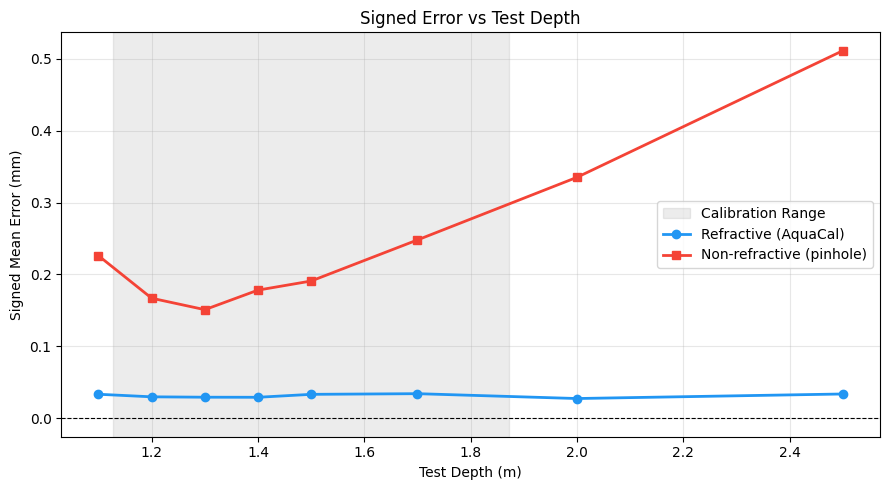
Signed Error vs Depth

The shaded region marks the calibration depth range. The refractive model maintains low, uniform error at all depths. The non-refractive model shows systematic depth-dependent bias because its wrong geometry produces scale errors that grow with distance from the water surface.

depths_plot = [r["depth"] for r in results_refr_exp2]
signed_refr = [r["signed_mean_mm"] for r in results_refr_exp2]
signed_nonrefr = [r["signed_mean_mm"] for r in results_nonrefr_exp2]

fig, ax = plt.subplots(figsize=(9, 5))
ax.axvspan(CALIB_DEPTH_RANGE[0], CALIB_DEPTH_RANGE[1], alpha=0.15, color="gray", label="Calibration Range")
ax.plot(depths_plot, signed_refr, marker="o", color=COLOR_REFRACTIVE, label=LABEL_REFRACTIVE, linewidth=2)
ax.plot(depths_plot, signed_nonrefr, marker="s", color=COLOR_NON_REFRACTIVE, label=LABEL_NON_REFRACTIVE, linewidth=2)
ax.axhline(0, color="black", linewidth=0.8, linestyle="--")
ax.set_xlabel("Test Depth (m)")
ax.set_ylabel("Signed Mean Error (mm)")
ax.set_title("Signed Error vs Test Depth")
ax.legend()
ax.grid(alpha=0.3)
plt.tight_layout()
plt.show()
plt.close()

rmse_refr = [r["rmse_mm"] for r in results_refr_exp2]
rmse_nonrefr = [r["rmse_mm"] for r in results_nonrefr_exp2]

fig, ax = plt.subplots(figsize=(9, 5))
ax.axvspan(CALIB_DEPTH_RANGE[0], CALIB_DEPTH_RANGE[1], alpha=0.15, color="gray", label="Calibration Range")
ax.plot(depths_plot, rmse_refr, marker="o", color=COLOR_REFRACTIVE, label=LABEL_REFRACTIVE, linewidth=2)
ax.plot(depths_plot, rmse_nonrefr, marker="s", color=COLOR_NON_REFRACTIVE, label=LABEL_NON_REFRACTIVE, linewidth=2)
ax.set_xlabel("Test Depth (m)")
ax.set_ylabel("Reconstruction RMSE (mm)")
ax.set_title("Reconstruction RMSE vs Test Depth")
ax.legend()
ax.grid(alpha=0.3)
plt.tight_layout()
plt.show()
plt.close()

max_rmse_refr = max(rmse_refr)
max_rmse_nonrefr = max(rmse_nonrefr)
print(f"Maximum RMSE across all test depths:")
print(f"  Refractive:     {max_rmse_refr:.2f} mm")
print(f"  Non-refractive: {max_rmse_nonrefr:.2f} mm")

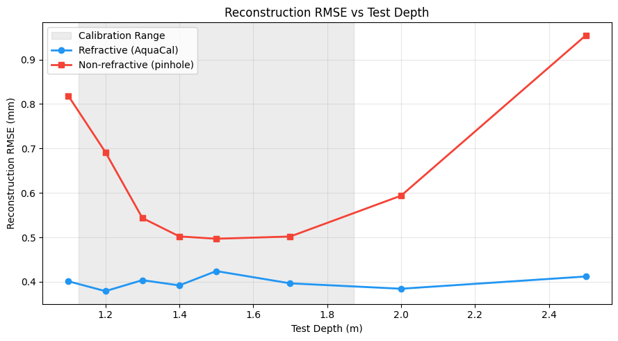
Maximum RMSE across all test depths:
  Refractive:     0.42 mm
  Non-refractive: 0.95 mm

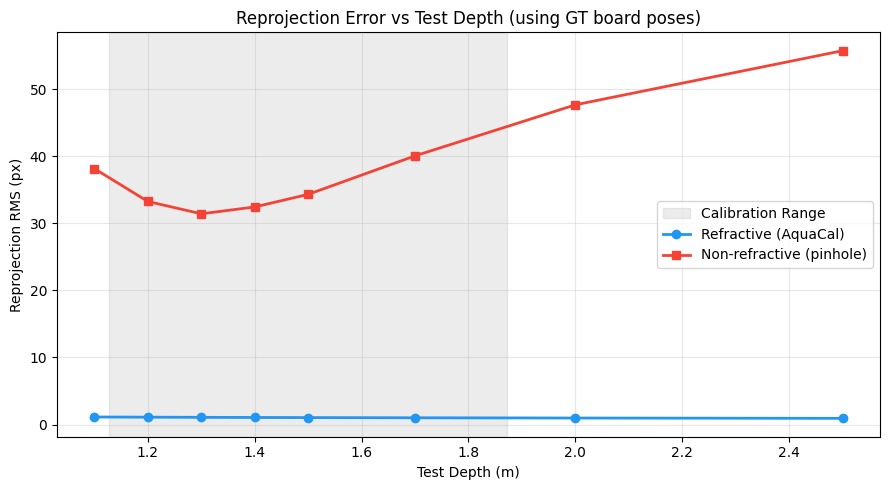
Reprojection Error vs Depth

Reprojection error measures how well the calibrated model explains the 2D observations at each test depth using the ground-truth board poses. Unlike 3D reconstruction error, this is a purely 2D metric — but it still degrades for the non-refractive model because refraction bends rays by a depth-dependent amount that a fixed pinhole model cannot accommodate.

reproj_refr = [r["reproj_rms_px"] for r in results_refr_exp2]
reproj_nonrefr = [r["reproj_rms_px"] for r in results_nonrefr_exp2]

fig, ax = plt.subplots(figsize=(9, 5))
ax.axvspan(CALIB_DEPTH_RANGE[0], CALIB_DEPTH_RANGE[1], alpha=0.15, color="gray", label="Calibration Range")
ax.plot(depths_plot, reproj_refr, marker="o", color=COLOR_REFRACTIVE, label=LABEL_REFRACTIVE, linewidth=2)
ax.plot(depths_plot, reproj_nonrefr, marker="s", color=COLOR_NON_REFRACTIVE, label=LABEL_NON_REFRACTIVE, linewidth=2)
ax.set_xlabel("Test Depth (m)")
ax.set_ylabel("Reprojection RMS (px)")
ax.set_title("Reprojection Error vs Test Depth (using GT board poses)")
ax.legend()
ax.grid(alpha=0.3)
plt.tight_layout()
plt.show()
plt.close()

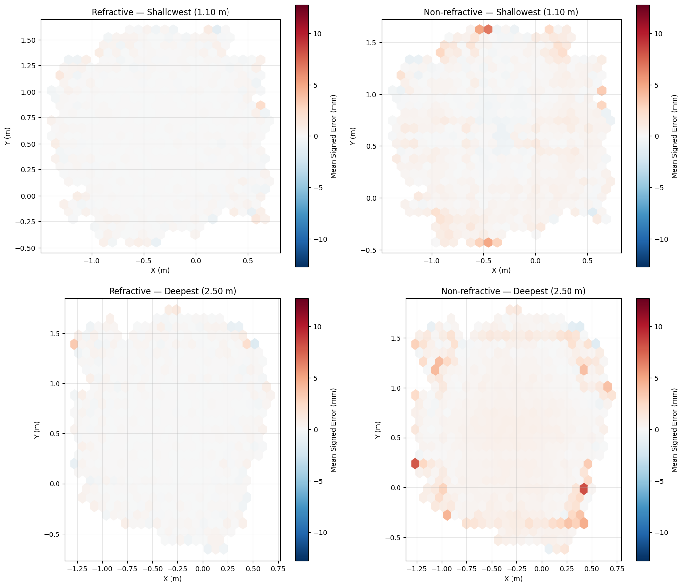
Spatial Error Distribution

Are reconstruction errors uniform across the field of view, or concentrated in certain regions? The heatmaps below show mean signed reconstruction error binned by XY position for the shallowest and deepest test depths.

The non-refractive model’s error is not only larger but spatially structured — it varies across the field of view because refraction angle depends on the incidence geometry, which a fixed pinhole distortion model cannot capture.

# Pick shallowest and deepest test depths for comparison
depth_indices = [0, len(TEST_DEPTHS) - 1]
depth_labels = ["Shallowest", "Deepest"]

fig, axes = plt.subplots(len(depth_indices), 2, figsize=(14, 6 * len(depth_indices)))

# Compute shared color scale across all panels
all_errors_mm = []
for di in depth_indices:
    for results in [results_refr_exp2, results_nonrefr_exp2]:
        sp = results[di]["spatial"]
        if sp is not None:
            all_errors_mm.extend((sp.signed_errors * 1000).tolist())
if all_errors_mm:
    vmax = max(abs(min(all_errors_mm)), abs(max(all_errors_mm)))
else:
    vmax = 1.0

# Hexbin gridsize: use equal x-y bin widths.  The data spans ~2*XY_EXTENT in
# both X and Y.  A gridsize of 25 gives bins of roughly 40 mm width, which is
# fine enough to show spatial structure without being too noisy.
HEXBIN_GRIDSIZE = 25

for row, (di, dlabel) in enumerate(zip(depth_indices, depth_labels)):
    depth_val = TEST_DEPTHS[di]
    for col, (results, model_label) in enumerate([
        (results_refr_exp2, "Refractive"),
        (results_nonrefr_exp2, "Non-refractive"),
    ]):
        ax = axes[row, col]
        sp = results[di]["spatial"]
        if sp is not None and len(sp.signed_errors) > 0:
            hb = ax.hexbin(
                sp.positions[:, 0], sp.positions[:, 1],
                C=sp.signed_errors * 1000,
                reduce_C_function=np.mean,
                gridsize=HEXBIN_GRIDSIZE,
                cmap="RdBu_r", vmin=-vmax, vmax=vmax,
                mincnt=1,
            )
            plt.colorbar(hb, ax=ax, label="Mean Signed Error (mm)")
        ax.set_xlabel("X (m)")
        ax.set_ylabel("Y (m)")
        ax.set_title(f"{model_label} — {dlabel} ({depth_val:.2f} m)")
        ax.set_aspect("equal")
        ax.grid(alpha=0.3)

plt.tight_layout()
plt.show()
plt.close()

scale_refr = [r["scale"] for r in results_refr_exp2]
scale_nonrefr = [r["scale"] for r in results_nonrefr_exp2]

fig, ax = plt.subplots(figsize=(9, 5))
ax.axvspan(CALIB_DEPTH_RANGE[0], CALIB_DEPTH_RANGE[1], alpha=0.15, color="gray", label="Calibration Range")
ax.plot(depths_plot, scale_refr, marker="o", color=COLOR_REFRACTIVE, label=LABEL_REFRACTIVE, linewidth=2)
ax.plot(depths_plot, scale_nonrefr, marker="s", color=COLOR_NON_REFRACTIVE, label=LABEL_NON_REFRACTIVE, linewidth=2)
ax.axhline(1.0, color="black", linewidth=0.8, linestyle="--", label="True scale (1.0)")
ax.set_xlabel("Test Depth (m)")
ax.set_ylabel("Scale Factor (measured / true)")
ax.set_title("Scale Factor vs Test Depth")
ax.legend()
ax.grid(alpha=0.3)
plt.tight_layout()
plt.show()
plt.close()

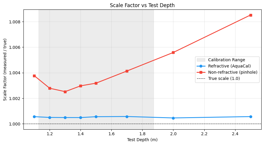
Experiment 2 Takeaway

The refractive model’s error stays low and uniform across all test depths — it learned the actual geometry and produces consistent 3D measurements regardless of depth. The non-refractive model’s error grows with depth because its biased focal lengths and camera positions produce scale distortions that worsen as targets move further from the cameras.

This is particularly important for applications where the measurement depth varies: animal tracking, reef surveys, or any scenario where targets move in depth.

Experiment 3: XY vs Z Precision Anisotropy

Question: Is reconstruction precision uniform in all directions, or does the camera geometry create a preferred axis?

When all cameras look straight down (optical axes parallel to Z), they have wide angular separation in XY — each camera views the same target from a different lateral position. But along Z (depth), all viewing angles are nearly identical. This creates anisotropic triangulation geometry: the system resolves XY position far more precisely than Z.

This geometric anisotropy affects both models, but the non-refractive model adds systematic Z bias from its wrong parameters on top. Using the same test data from Experiment 2, we decompose triangulation error into lateral (XY) and depth (Z) components to quantify both effects.

print("=== Experiment 3: XY vs Z Precision Anisotropy ===")
print("Reusing test data from Experiment 2\n")

# For each test depth, triangulate corners and compare to ground truth positions.
# Decompose the 3D position error into XY (lateral) and Z (depth) components.

def compute_xyz_errors(calibration, test_poses, test_detections, board):
    """Triangulate corners, compare to GT, return per-depth XY/Z error arrays."""
    results = []
    poses_by_frame = {bp.frame_idx: bp for bp in test_poses}

    xy_errors = []
    z_errors = []
    signed_z_errors = []

    for frame_idx in test_detections.frames:
        tri_corners = triangulate_charuco_corners(calibration, test_detections, frame_idx)
        if not tri_corners:
            continue

        bp = poses_by_frame[frame_idx]
        R_board, _ = cv2.Rodrigues(bp.rvec)

        for corner_id, tri_pos in tri_corners.items():
            if corner_id not in board.corner_positions:
                continue
            p_board = board.corner_positions[corner_id]
            p_gt = R_board @ p_board + bp.tvec

            err = tri_pos - p_gt
            xy_errors.append(np.linalg.norm(err[:2]))
            z_errors.append(abs(err[2]))
            signed_z_errors.append(err[2])

    xy_arr = np.array(xy_errors)
    z_arr = np.array(z_errors)
    signed_z_arr = np.array(signed_z_errors)
    xy_rmse = np.sqrt(np.mean(xy_arr**2))
    z_rmse = np.sqrt(np.mean(z_arr**2))
    ratio = z_rmse / xy_rmse if xy_rmse > 0 else float("inf")

    return {
        "xy_rmse_mm": xy_rmse * 1000,
        "z_rmse_mm": z_rmse * 1000,
        "xy_mean_signed_mm": np.mean(xy_arr) * 1000,
        "z_mean_signed_mm": np.mean(signed_z_arr) * 1000,
        "ratio": ratio,
        "xy_errors_mm": xy_arr * 1000,
        "z_errors_mm": z_arr * 1000,
        "n_points": len(xy_errors),
    }


exp3_refr = []
exp3_nonrefr = []

for i, depth in enumerate(TEST_DEPTHS):
    test_poses = exp2_test_poses[i]
    test_detections = exp2_test_detections[i]

    r_refr = compute_xyz_errors(result_refr, test_poses, test_detections, board_exp2)
    r_nonrefr = compute_xyz_errors(result_nonrefr, test_poses, test_detections, board_exp2)
    r_refr["depth"] = depth
    r_nonrefr["depth"] = depth
    exp3_refr.append(r_refr)
    exp3_nonrefr.append(r_nonrefr)

    print(f"  Z = {depth:.2f} m:")
    print(f"    Refractive:     XY = {r_refr['xy_rmse_mm']:.3f} mm, "
          f"Z = {r_refr['z_rmse_mm']:.3f} mm, ratio = {r_refr['ratio']:.1f}x")
    print(f"    Non-refractive: XY = {r_nonrefr['xy_rmse_mm']:.3f} mm, "
          f"Z = {r_nonrefr['z_rmse_mm']:.3f} mm, ratio = {r_nonrefr['ratio']:.1f}x")

print("\nAnisotropy analysis complete.")

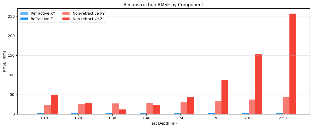
XY vs Z RMSE across Depth

The grouped bar chart below compares lateral (XY) and depth (Z) reconstruction RMSE for both models at each test depth. The refractive model shows the baseline geometric anisotropy; the non-refractive model amplifies it with systematic Z bias from its wrong parameters.

depths_exp3 = [r["depth"] for r in exp3_refr]
x_pos = np.arange(len(depths_exp3))
w = 0.2  # bar width

fig, ax = plt.subplots(figsize=(12, 5))
ax.bar(x_pos - 1.5 * w, [r["xy_rmse_mm"] for r in exp3_refr], w,
       label="Refractive XY", color=COLOR_REFRACTIVE, alpha=0.7)
ax.bar(x_pos - 0.5 * w, [r["z_rmse_mm"] for r in exp3_refr], w,
       label="Refractive Z", color=COLOR_REFRACTIVE)
ax.bar(x_pos + 0.5 * w, [r["xy_rmse_mm"] for r in exp3_nonrefr], w,
       label="Non-refractive XY", color=COLOR_NON_REFRACTIVE, alpha=0.7)
ax.bar(x_pos + 1.5 * w, [r["z_rmse_mm"] for r in exp3_nonrefr], w,
       label="Non-refractive Z", color=COLOR_NON_REFRACTIVE)
ax.set_xlabel("Test Depth (m)")
ax.set_ylabel("RMSE (mm)")
ax.set_title("Reconstruction RMSE by Component")
ax.set_xticks(x_pos)
ax.set_xticklabels([f"{d:.2f}" for d in depths_exp3])
ax.legend(ncol=2)
ax.grid(axis="y", alpha=0.3)
plt.tight_layout()
plt.show()
plt.close()

Anisotropy Ratio vs Depth

The ratio Z_RMSE / XY_RMSE quantifies how many times worse depth precision is compared to lateral precision. A ratio of 1 would indicate isotropic precision; higher values indicate a “cigar-shaped” error distribution elongated along Z.

Both models show anisotropy from the rig geometry, but the non-refractive model’s ratio is higher because its systematic Z bias adds to the geometric limitation.

ratios_refr = [r["ratio"] for r in exp3_refr]
ratios_nonrefr = [r["ratio"] for r in exp3_nonrefr]

fig, ax = plt.subplots(figsize=(9, 5))
ax.axvspan(CALIB_DEPTH_RANGE[0], CALIB_DEPTH_RANGE[1], alpha=0.15, color="gray", label="Calibration Range")
ax.plot(depths_exp3, ratios_refr, marker="o", color=COLOR_REFRACTIVE,
        label=LABEL_REFRACTIVE, linewidth=2)
ax.plot(depths_exp3, ratios_nonrefr, marker="s", color=COLOR_NON_REFRACTIVE,
        label=LABEL_NON_REFRACTIVE, linewidth=2)
ax.axhline(1.0, color="black", linewidth=0.8, linestyle="--", label="Isotropic (ratio = 1)")
ax.set_xlabel("Test Depth (m)")
ax.set_ylabel("Z RMSE / XY RMSE")
ax.set_title("Depth-to-Lateral Precision Ratio vs Test Depth")
ax.legend()
ax.grid(alpha=0.3)
plt.tight_layout()
plt.show()
plt.close()

print(f"Anisotropy ratio (refractive):     {min(ratios_refr):.1f}x – {max(ratios_refr):.1f}x "
      f"(mean {np.mean(ratios_refr):.1f}x)")
print(f"Anisotropy ratio (non-refractive): {min(ratios_nonrefr):.1f}x – {max(ratios_nonrefr):.1f}x "
      f"(mean {np.mean(ratios_nonrefr):.1f}x)")

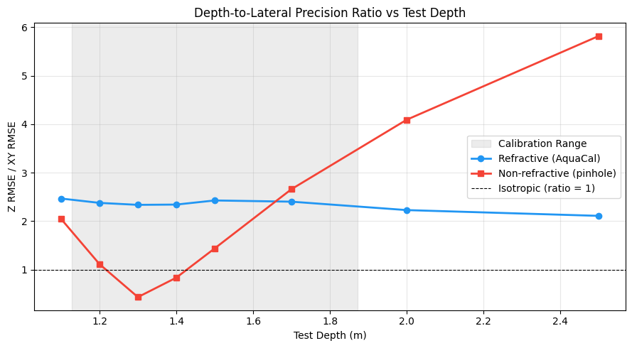
Anisotropy ratio (refractive):     2.1x – 2.5x (mean 2.3x)
Anisotropy ratio (non-refractive): 0.4x – 5.8x (mean 2.3x)

Error Distribution: Shallowest vs Deepest

Violin plots show the full distribution of per-point errors at the shallowest and deepest test depths for both models. The non-refractive model’s Z distribution is dramatically wider — its systematic bias stacks on top of the geometric anisotropy that both models share.

# 2x2 grid: rows = shallowest/deepest, cols = refractive/non-refractive
shallow_refr, deep_refr = exp3_refr[0], exp3_refr[-1]
shallow_nonrefr, deep_nonrefr = exp3_nonrefr[0], exp3_nonrefr[-1]

fig, axes = plt.subplots(2, 2, figsize=(12, 9), sharey=True)

panels = [
    (axes[0, 0], shallow_refr, f"Refractive — {shallow_refr['depth']:.2f} m"),
    (axes[0, 1], shallow_nonrefr, f"Non-refractive — {shallow_nonrefr['depth']:.2f} m"),
    (axes[1, 0], deep_refr, f"Refractive — {deep_refr['depth']:.2f} m"),
    (axes[1, 1], deep_nonrefr, f"Non-refractive — {deep_nonrefr['depth']:.2f} m"),
]

for ax, result, label in panels:
    data = [result["xy_errors_mm"], result["z_errors_mm"]]
    parts = ax.violinplot(data, positions=[0, 1], showmedians=True, showextrema=False)

    for pc, color in zip(parts["bodies"], ["#4CAF50", "#FF9800"]):
        pc.set_facecolor(color)
        pc.set_alpha(0.7)
    parts["cmedians"].set_color("black")

    ax.set_xticks([0, 1])
    ax.set_xticklabels(["XY Error", "Z Error"])
    ax.set_title(label)
    ax.grid(axis="y", alpha=0.3)

axes[0, 0].set_ylabel("Absolute Error (mm)")
axes[1, 0].set_ylabel("Absolute Error (mm)")
fig.text(0.01, 0.73, "Shallowest", va="center", rotation="vertical", fontsize=12, fontweight="bold")
fig.text(0.01, 0.28, "Deepest", va="center", rotation="vertical", fontsize=12, fontweight="bold")
fig.suptitle("Per-Point Error Distributions", fontsize=13, y=1.01)
plt.tight_layout()
plt.show()
plt.close()

print(f"Shallowest ({shallow_refr['depth']:.2f} m):")
print(f"  Refractive     — XY median: {np.median(shallow_refr['xy_errors_mm']):.3f} mm, "
      f"Z median: {np.median(shallow_refr['z_errors_mm']):.3f} mm")
print(f"  Non-refractive — XY median: {np.median(shallow_nonrefr['xy_errors_mm']):.3f} mm, "
      f"Z median: {np.median(shallow_nonrefr['z_errors_mm']):.3f} mm")
print(f"Deepest ({deep_refr['depth']:.2f} m):")
print(f"  Refractive     — XY median: {np.median(deep_refr['xy_errors_mm']):.3f} mm, "
      f"Z median: {np.median(deep_refr['z_errors_mm']):.3f} mm")
print(f"  Non-refractive — XY median: {np.median(deep_nonrefr['xy_errors_mm']):.3f} mm, "
      f"Z median: {np.median(deep_nonrefr['z_errors_mm']):.3f} mm")

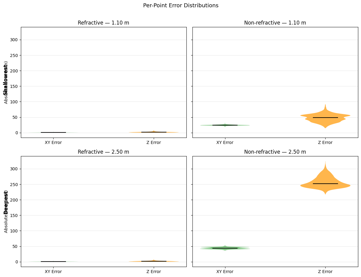
Shallowest (1.10 m):
  Refractive     — XY median: 0.667 mm, Z median: 1.293 mm
  Non-refractive — XY median: 24.034 mm, Z median: 48.312 mm
Deepest (2.50 m):
  Refractive     — XY median: 0.849 mm, Z median: 1.341 mm
  Non-refractive — XY median: 43.759 mm, Z median: 252.402 mm

Experiment 3 Takeaway

Reconstruction precision is highly anisotropic: Z (depth) errors are consistently larger than XY (lateral) errors for both models. The refractive model shows the baseline geometric anisotropy — an inherent consequence of the downward-looking camera arrangement where all cameras share a similar viewing angle along Z. The non-refractive model makes it worse: its systematic parameter bias amplifies Z error while leaving XY relatively unchanged, producing even higher anisotropy ratios.

Practical implications:

• XY tracking (e.g. horizontal position of fish) is inherently precise with either model

• Depth estimation (Z) is the limiting factor — and the non-refractive model makes it substantially worse

• Applications that only need 2D plan-view tracking can expect significantly better precision than the overall 3D RMSE suggests

• For depth-critical applications, use the refractive model and consider adding cameras at oblique angles to improve Z triangulation geometry

Exported Data

The CSVs below capture the per-record data behind all plots in this notebook, so downstream consumers can reproduce statistics and figures without running AquaCal.

# --- Exp1: per-camera parameter errors ---
# Compute mean Z shift of free cameras for mean-shift correction
_free = [c for c in camera_names if c != camera_names[0]]
_mz = {
    "refractive": np.mean([errors_refr[c]["z_position_error_mm"] for c in _free]),
    "non_refractive": np.mean([errors_nonrefr[c]["z_position_error_mm"] for c in _free]),
}

rows_exp1 = []
for cam in camera_names:
    for label, errors, result in [
        ("refractive", errors_refr, result_refr),
        ("non_refractive", errors_nonrefr, result_nonrefr),
    ]:
        C_gt = scenario.extrinsics[cam].C
        C_est = result.cameras[cam].extrinsics.C
        rows_exp1.append({
            "camera": cam,
            "model": label,
            "focal_length_error_pct": errors[cam]["focal_length_error_pct"],
            "z_position_error_mm": errors[cam]["z_position_error_mm"] - _mz[label],
            "xy_position_error_mm": errors[cam]["xy_position_error_mm"],
            "gt_x_m": C_gt[0], "gt_y_m": C_gt[1], "gt_z_m": C_gt[2],
            "est_x_m": C_est[0], "est_y_m": C_est[1], "est_z_m": C_est[2],
            "reprojection_rms_px": result.diagnostics.reprojection_error_rms,
        })
df_exp1 = pd.DataFrame(rows_exp1)

# --- Exp2: depth-generalization metrics ---
rows_exp2 = []
for r_refr, r_nonrefr in zip(results_refr_exp2, results_nonrefr_exp2):
    for label, r in [("refractive", r_refr), ("non_refractive", r_nonrefr)]:
        rows_exp2.append({
            "test_depth_m": r["depth"],
            "model": label,
            "signed_mean_mm": r["signed_mean_mm"],
            "rmse_mm": r["rmse_mm"],
            "scale_factor": r["scale"],
            "calib_depth_min_m": CALIB_DEPTH_RANGE[0],
            "calib_depth_max_m": CALIB_DEPTH_RANGE[1],
        })
df_exp2 = pd.DataFrame(rows_exp2)

# --- Exp2: spatial error distribution (positions + signed errors per depth) ---
rows_spatial = []
for r_refr, r_nonrefr in zip(results_refr_exp2, results_nonrefr_exp2):
    for label, r in [("refractive", r_refr), ("non_refractive", r_nonrefr)]:
        sp = r["spatial"]
        if sp is not None and len(sp.signed_errors) > 0:
            for i in range(len(sp.signed_errors)):
                rows_spatial.append({
                    "test_depth_m": r["depth"],
                    "model": label,
                    "x_m": sp.positions[i, 0],
                    "y_m": sp.positions[i, 1],
                    "z_m": sp.positions[i, 2],
                    "signed_error_mm": sp.signed_errors[i] * 1000,
                })
df_spatial = pd.DataFrame(rows_spatial)

# --- Exp3: XY vs Z anisotropy ---
rows_exp3 = []
for r_refr, r_nonrefr in zip(exp3_refr, exp3_nonrefr):
    for label, r in [("refractive", r_refr), ("non_refractive", r_nonrefr)]:
        rows_exp3.append({
            "test_depth_m": r["depth"],
            "model": label,
            "xy_rmse_mm": r["xy_rmse_mm"],
            "z_rmse_mm": r["z_rmse_mm"],
            "xy_mean_signed_mm": r["xy_mean_signed_mm"],
            "z_mean_signed_mm": r["z_mean_signed_mm"],
            "anisotropy_ratio": r["ratio"],
            "n_points": r["n_points"],
        })
df_exp3 = pd.DataFrame(rows_exp3)

# --- Write CSVs ---
OUTPUT_DIR.mkdir(parents=True, exist_ok=True)
path_exp1 = OUTPUT_DIR / "exp1_parameter_errors.csv"
path_exp2 = OUTPUT_DIR / "exp2_depth_generalization.csv"
path_spatial = OUTPUT_DIR / "exp2_spatial_errors.csv"
path_exp3 = OUTPUT_DIR / "exp3_xy_vs_z_anisotropy.csv"
df_exp1.to_csv(path_exp1, index=False)
df_exp2.to_csv(path_exp2, index=False)
df_spatial.to_csv(path_spatial, index=False)
df_exp3.to_csv(path_exp3, index=False)

print(f"Wrote {path_exp1}  ({len(df_exp1)} rows)")
print(f"Wrote {path_exp2}  ({len(df_exp2)} rows)")
print(f"Wrote {path_spatial}  ({len(df_spatial)} rows)")
print(f"Wrote {path_exp3}  ({len(df_exp3)} rows)")

Summary

Three experiments, one calibration:

Experiment	What we tested	Key finding
1 — Parameter Fidelity	Same data, two models	Non-refractive absorbs refraction into focal length and position bias
2 — Depth Generalization	Same calibration, sweep test depth	Non-refractive error grows with depth; refractive stays flat
3 — XY vs Z Anisotropy	Decompose error by direction	Z error dominates XY for both models; non-refractive amplifies the gap

When is refractive calibration essential?

• Camera-to-water distance is significant (>= 0.3 m)

• Measurement depth varies across sessions or within a session

• High 3D accuracy is required (< 5 mm)

• You need stable calibration across depth ranges

When might pinhole be acceptable?

• Cameras are very close to the water surface (< 0.1 m)

• Only 2D detection or tracking is needed (no 3D reconstruction)

• Accuracy requirements are very relaxed (> 20 mm)

• Data collection depth is constant and pre-known

---

Further reading:

• Full pipeline tutorial — calibrate a rig end-to-end

• Theory documentation — refractive geometry model and Snell’s law derivation

• Optimizer guide — tuning the Stage 3 bundle adjustment